
Regional Gravity Survey of Silver Spurs Ranch
Wes Wilson
Sangre Geophysics
November 2, 2006
Disclaimer:
Opinions expressed are solely those of the author and do not reflect those of the
Silver Spurs Property Owners Association.

2
Motivation
The geology of the Spanish Peaks area is unique. Emplacement of the Spanish Peaks created a
series of radial faults which allowed the formation of dikes that permeate the region.
Many ground water systems are fracture controlled. Dikes and associated fracture patterns create
a complex water flow regime where groundwater flow is redirected by impermeable dikes. By
understanding large scale fractures and subsurface dike locations, connected regions of water flow
can be identified.
The purpose of this study is to establish whether or not the Spanish Peak dikes extend into Silver
Spurs Ranch, and if so, where are they and at what depth. Results are evaluated to determine
possible connected water flow regions and possible areas of recharge where the water flow is
replenished.
A geophysical gravity survey is a relatively inexpensive method for mapping the subsurface of large
regional areas. This report presents the results of a regional gravity survey conducted over the
Silver Spurs Ranch in June, 2006.
Regional geology
The surface geology of the Spanish Peaks area has been strongly influenced by the formation of
the Spanish Peaks. The Spanish Peaks are thought to be large intruded magma bodies called
stocks or batholiths. These bodies formed at depth some 27 million years ago and gradually
became visible as the softer overlying rock eroded away.
When the Spanish Peak stocks were formed, vertical forces of the hot rock caused fractures to form
in the overlying sedimentary rocks. As the fractures were created, hot magma flowed into the
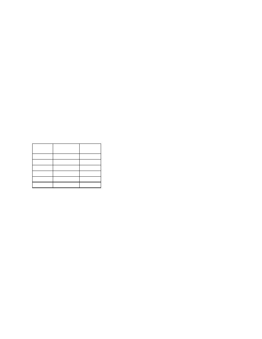
cracks to form the dikes. Figure 1 shows an outcrop of a typical dike just north of the town of La
Veta. Typical widths of the dikes range from a few meters to tens of meters.
Simple mathematical models based on point stresses in thin plates predict the expected fracture
pattern for such an emplacement to be radial arcs. These arcs curve at the ends to align with
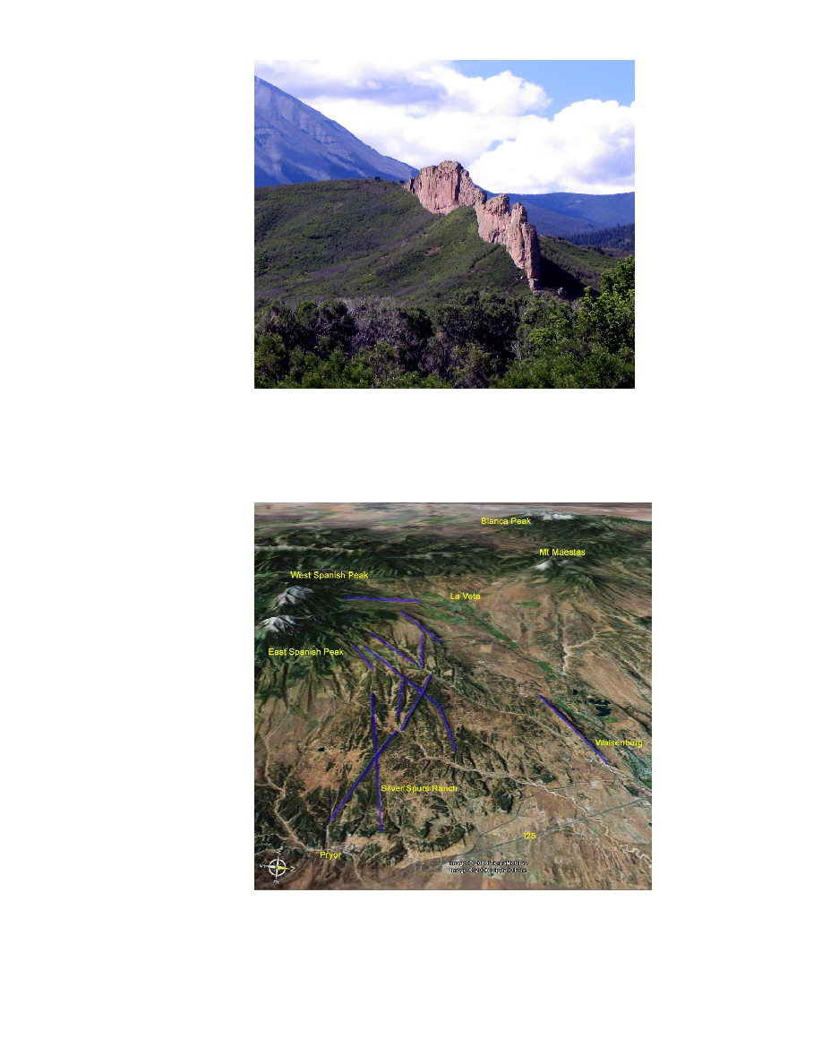
existing horizontal stress in the plate. Figure 2 shows the Spanish Peaks as seen from a point of
view above Silver Spurs Ranch looking west. Major dikes are outlined in blue to emphasize their
radial nature. Not all dikes follow the same radial pattern. This suggests that the dikes most likely
formed over a period time under different stress conditions.
Horizontal and vertical stresses associated with the dikes also left an imprint of vertical faults in the
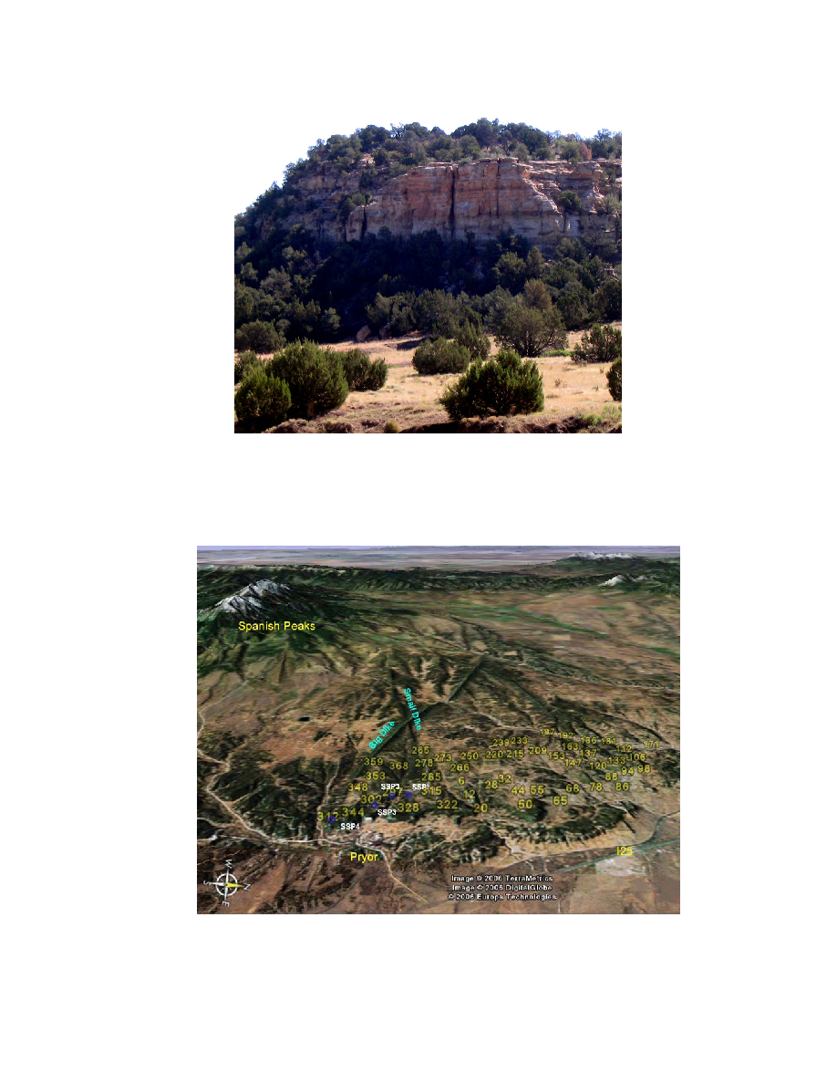
weaker overlying sedimentary layers. Figure 3 shows vertical factures in the Trinidad sandstone
formation, a rock layer found beneath Silver Spurs Ranch.
Dikes and vertical fracturing control water flow through out the region. The ability of water to flow
through rock is measured as permeability. Permeability of the dike rock is higher than the
surrounding sedimentary rock. When water flow encounters a buried dike, it is diverted along the
vertical plane of the dike. Water flowing in sedimentary rocks will seek out channels provided by
existing vertical fractures. The combination of dikes and fractures creates a complex water flow
pattern in the region. By understanding the location of the dikes both above and below the surface,
water barriers created by dikes can be outlined to understand water flow patterns.
The physical properties of the dike rock that create higher permeability also make the rock heavier
or denser. Surrounding sedimentary rock is less dense than the dike rock. A gravity survey takes
advantage of the density contrast to map the location of the subsurface dikes.
3
Gravity survey design
A gravity survey measures the pull of gravity at various survey locations. The pull of gravity varies
as a function of rock density. Gravity differences on the surface of the earth are small but
measurable. Refer to Appendix C for a detailed description of the gravity exploration method as
presented by the United States Geological Survey (USGS).
A gravity survey is one of the most inexpensive geophysical techniques for mapping the
subsurface. The survey is conducted by taking a series of measurements over the survey area. A
regional gravity survey was conducted on Silver Spurs Ranch over the period June 16 - 20, 2006.
Gravity measurements were taken along existing roads at a spacing of 100 meters (m). This
resulted in 368 measurements along 36.8 linear kilometers (23 miles). The survey covered
approximately 31 square kilometers (12 square miles). Measurement locations are shown with
respect to the Spanish Peaks in Figure 4.
To determine density contrast, rock samples were taken from several locations on Silver Spurs
Ranch (The Ranch). Densities for rock sample locations shown in Figure 4 are listed in Table 1.
Samples WAL1 and WAL2 are taken from a dike outcrop along Highway 85 north of Walsenburg.
They indicate an average dike density of 3.85 grams per cubic centimeter (g/cc).
site
rock type
density
g/cc
WAL1
hornblende
4.09
WAL2
hornblende
3.60
SSP1
sandstone
2.36
SSP2
sandstone
2.37
SSP3
sandstone
2.63
SSP4
sandstone
2.37
Table 1 Rock sample density measurements.
The average density of the 4 sandstone samples is 2.43 g/cc. A density difference of 1.42 g/cc
between the sandstone and dike rocks is large enough to create a change in gravity that can be
measured by an exploration gravity meter.
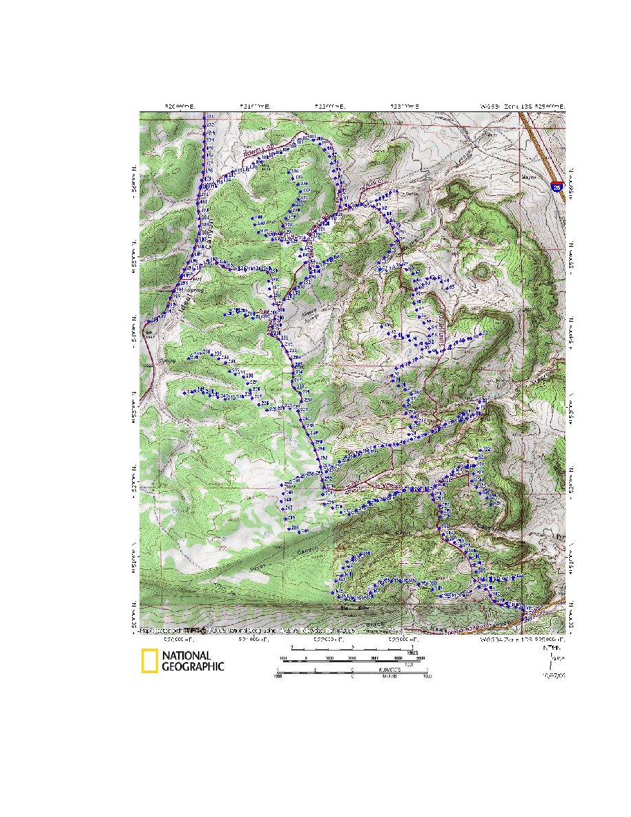
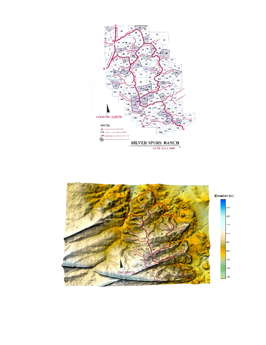
Gravity surface locations are displayed on a USGS topographical map in Figure 5. Universal
Transversal Mercator (UTM) coordinates are annotated along the map axes. Gravity station (stn)
locations and the corresponding UTM coordinates (XYs) are listed in Appendix B.
Roads on the USGS maps are taken from an older vintage aerial photo and the road locations vary
from their present day locations as shown by gravity survey markers along current roads. For
reference, the property map, Figure 6, will be shown with the gravity maps. The property map is
shown with a digital elevation map in Figure 7.
Gravity measurement
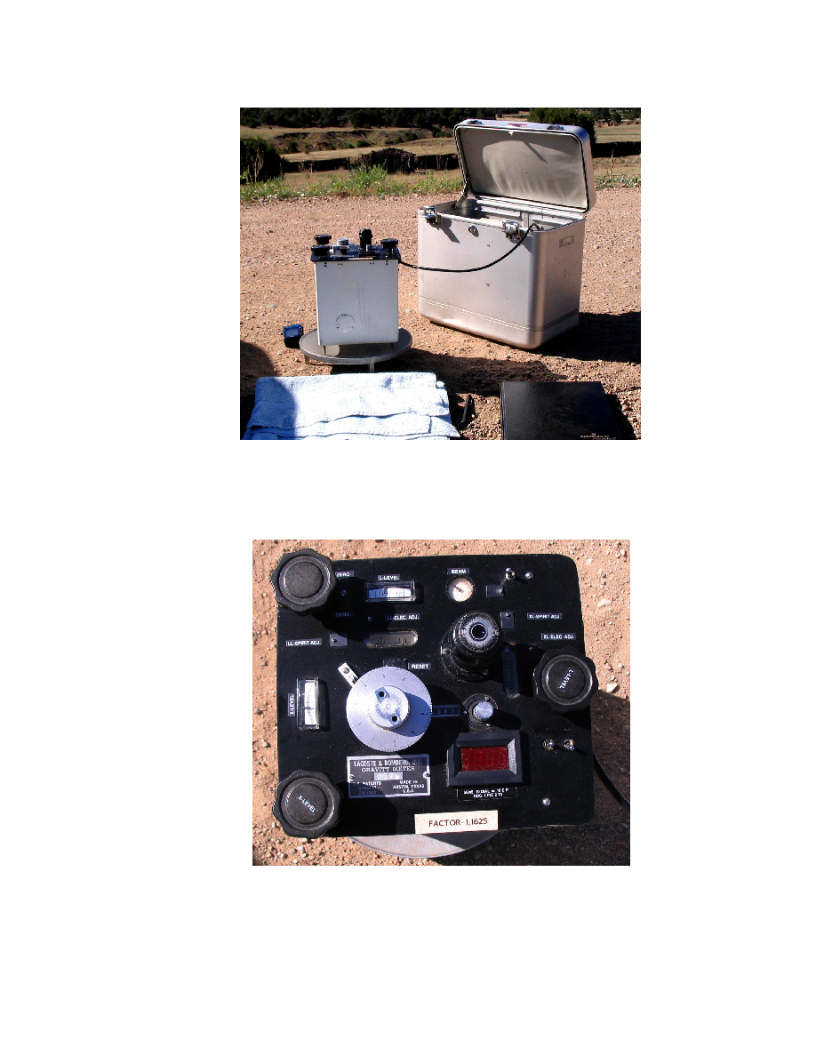
At each survey location a gravity measurement is made along with latitude, longitude and elevation.
Layout for a typical gravity measurement is shown in Figure 8. The gravity meter is about the size
of a car battery and is shown with the aluminum carrying case. The carrying case contains a
battery which powers the temperature control and readout displays. The top view of the gravity
meter shows the controls, Figure 9. A measurement is made by first setting the meter on a tripod

4
base. The instrument is leveled using the large knobs on the left side corners and middle right.
Once level, the aluminum dial is rotated until the `beam' galvanometer in the upper right reads zero
or is straight up. Gravity values are then read off the aluminum dial.
Once the gravity value is read, the latitude, longitude and elevation are read from the Garmin GPS
receiver shown at the upper left in Figure 8. The latitude/longitude GPS coordinates were read to
within an accuracy of about 10-20 meters. Vertical measurements of elevation were accurate to
20m at best. For a gravity survey, accurate vertical elevation measurements are critical for
determining gravity corrections. To improve vertical accuracy, the latitude/longitude locations for
each measurement were used to locate the corresponding elevation on the USGS map in Figure 5.
The Garmin GPS receiver and the USGS map use the WGS84 projection. Elevations (elev) in
meters for each location are listed in Appendix B.
Measurements are noted in the black survey book, the meter is locked and set into the aluminum
carrying case, equipment is loaded into the truck and the next survey location is found by driving
along the road 100m using the GPS receiver for reference. Each measurement took from 4-8
minutes.
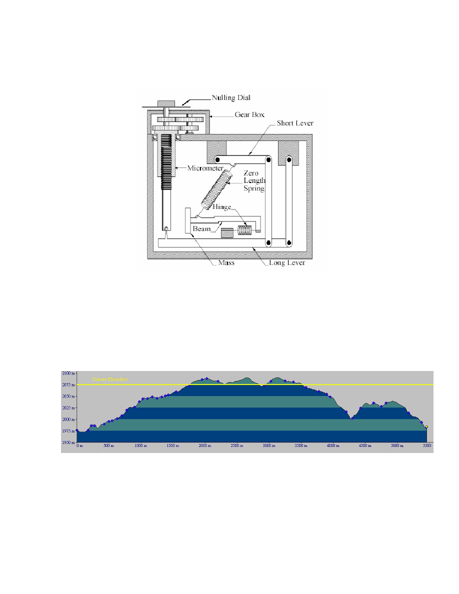
A cross section of the gravity meter is shown in Figure 10. The gravity meter contains a sensitive
spring which balances an internal mass on a beam. The mass is balanced by turning the nulling
dial which corresponds with the aluminum dial shown in Figure 9. The gravity meter used for the
survey was a Lacoste and Romberg D meter with a sensitivity of about .1 mgal gravity units. For
reference, the surface gravity along the equator of the earth is about 1 million mgal. The gravity
meter measures to less than 1 part per million of the total gravity field.
Gravity corrections
A number of factors influence a gravity measurement. When the gravity survey is corrected for
known variations, the resulting gravity map shows the unknown or anomalous gravity. Gravity
anomalies are modeled mathematically based on known density variations to determine possible
subsurface bodies or, in this case, dike locations.
Gravity measurements are affected by the following known factors:
·
Electronic instrument drift during the course of the survey
·
Tidal variation caused by the sun and moon
·
Latitude variations caused by the shape of the earth
·
Elevation differences along the survey profile
·
Density difference beneath a corrected datum elevation
·
Elevation differences in the surrounding terrain
Electronic instrument drift occurs in any electronic instrument. Instrument heating, stray
capacitance and other factors cause a measuring device to change slightly over time. The gravity
meter is no exception. To correct for instrument drift, base stations are established during the
survey as reference points. A base station measurement is made, several gravity station
measurements are made and then the base station is re-measured to identify any instrument drift.
For this survey, a base station was re-measured every 2 hours at a maximum. Instrument drift is
assumed to be linear between stations and is removed from the measurements. Details of each
correction are summarized in Appendix A.
Tidal pull of the sun and moon also affect the gravity measurement. Tidal corrections can be
computed mathematically, but in general the variation is assumed to be linear over the time frame
of the drift correction. The correction is applied at the same time as the drift correction. Appendix B
shows the actual field reading from the gravity meter, `field g', in gravity meter units. The `rel g'
column shows the relative gravity value in mgal units with the drift corrections applied. The survey

5
base station was established on the SE corner of the driveway at 463 Leather Dr. To find absolute
gravity measurements the `rel g' value is added to a known gravity station established by the US
Geodetic Survey. Such a station exists at Trinidad Junior College and a measurement was made
for completeness of the survey. However, when looking for anomalies, only the change in gravity is
needed. Therefore, relative gravity changes are used for interpretation.
Gravity is caused by presence of mass. Any object with mass has a gravitational attraction. As
one moves away from the mass, the gravitational attraction decreases. The same is true for the
earth. As one moves away from the earth, the gravitational attraction decreases. The earth is not
completely solid and as the earth turns, the centrifugal force causes the earth to bulge along the
equator. The bulge causes the surface of the earth to be farther away from the center of the earth
at the equator than at the poles. This causes the measured gravity to be lower at the equator than
at the poles. The change is a function of the shape of the earth, and the shape is well known from
satellite measurements. The correction is known as a latitude correction formally defined as the
International Association of Geodesy Reference System 1980. Gravity measurements with the
applied latitude correction are listed in the column marked `latitude' in Appendix B.
Elevation change causes a change in gravity. An elevation profile along Silver Spurs Rd from north
to south, Figure 11, shows an elevation variation of approximately 170m. For an average density of
2.67 g/cc, this elevation difference results in a gravity change of 50 mgals. Since the dike
anomalies are less than 10 mgals, an elevation correction must be made to the field
measurements. The correction is called a free air correction. The `free air' column in Appendix B
shows the gravity measurements which have been corrected for drift, latitude and elevation. These
measurements are referenced to a constant elevation datum of 2076 m, the elevation of the base
station.
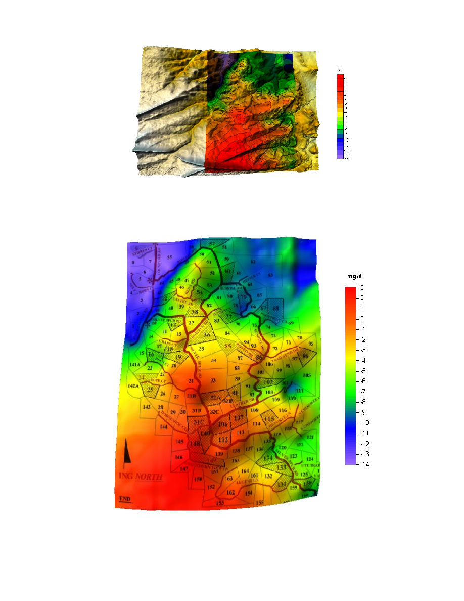
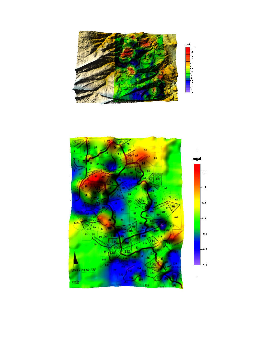
The free air gravity values are contoured to generate a free air anomaly map, Figure 13. The
anomaly map is shown with the digital elevation map in Figure 12. Color contours are in gravity
units of mgal shown annotated on the color bar. The free air anomaly map generally follows the
topography. Figure 12 shows gravity highs in red roughly following the elevation highs along the
ridges found on The Ranch.
Two additional corrections are necessary before attempting an interpretation, the Bouguer
correction and the terrain correction. The free air correction compensates for elevation variations
with reference to a datum elevation. The Bouguer correction adjusts the gravity measurements to
fill in the surface below the datum and removes the surface above the datum. The resulting gravity
measurement is as if it was measured on a flat surface at the datum elevation. The Bouguer
correction is combined with the free air correction to generate the `bouger' values in Appendix B.
The corresponding Bouguer anomaly map is seen in Figures 14 and 15.
The Bouguer anomaly map highlights regions of excess mass. A large positive anomaly of 3 mgal
is seen around properties 39 and 40 along Silver Spur Rd. Although large, it is smaller than the
free air anomaly of 11 mgals at the same location. There does not appear to be a direct correlation
of the anomalies with the topography. This suggests that a gravity correction related to the
surrounding terrain may be necessary.
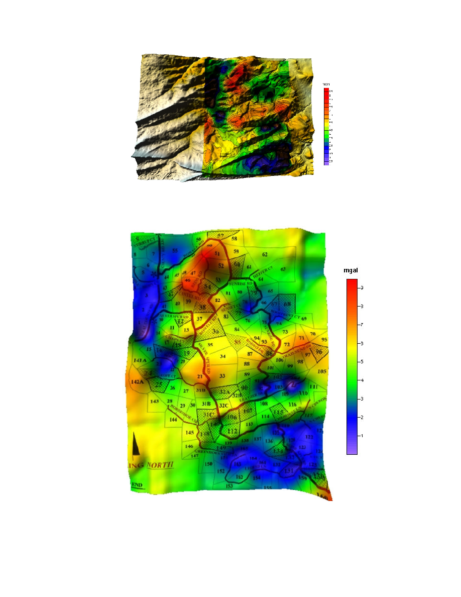
The complete Bouguer anomaly maps, Figures 16 and 17, take into account terrain corrections
about each gravity measurement. Appendix B lists the anomaly values in the column marked
`complete.' The complete Bouguer anomaly map shows a general correlation with topography as
expected and will form the basis of the gravity interpretation.
Gravity modeling
The complete Bouguer anomaly map shows remaining gravity variations after all corrections are
made. Anomalies associated with the near subsurface geology are interpreted by matching a

6
computed gravity field above blocky models to the observed gravity anomaly. When the field
matches, one possible solution has been determined. The technique is referred to interchangeably
as either `modeling' or `interpretation.'
The gravity field for simple geometric structures like rectangles and n-sided polygons can be
computed for a given density. To simplify the gravity modeling, the subsurface can be assumed to
be 2 dimensional (2D). This assumption gives a good approximation when the 2D cross section is
taken perpendicular to the trend of the gravity anomaly. A 3D approximation is made by assuming
that the 2D model continues into and out of the plane. This is called a 2.5D approximation. To
visualize, one can consider a loaf of bread. The slice of bread in the center of the loaf would be the
2D model and the entire loaf of bread would be the 2.5D model.
Gravity modeling was accomplished with Geomodel, a modeling software package. The program
allows a user to interactively define 2.5D geometric blocks to match the observed gravity anomaly.
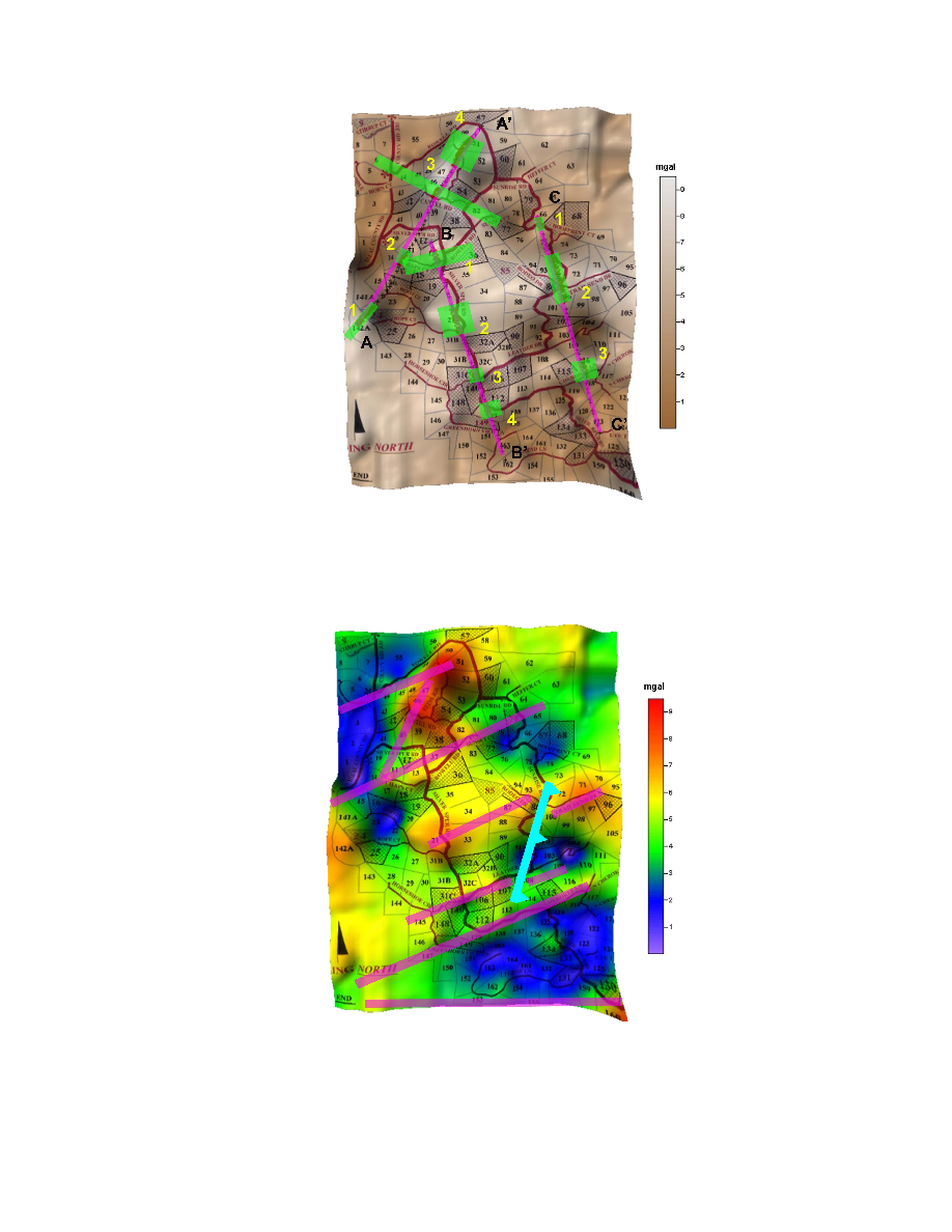
Block vertices can be adjusted interactively to refine the interpretation.
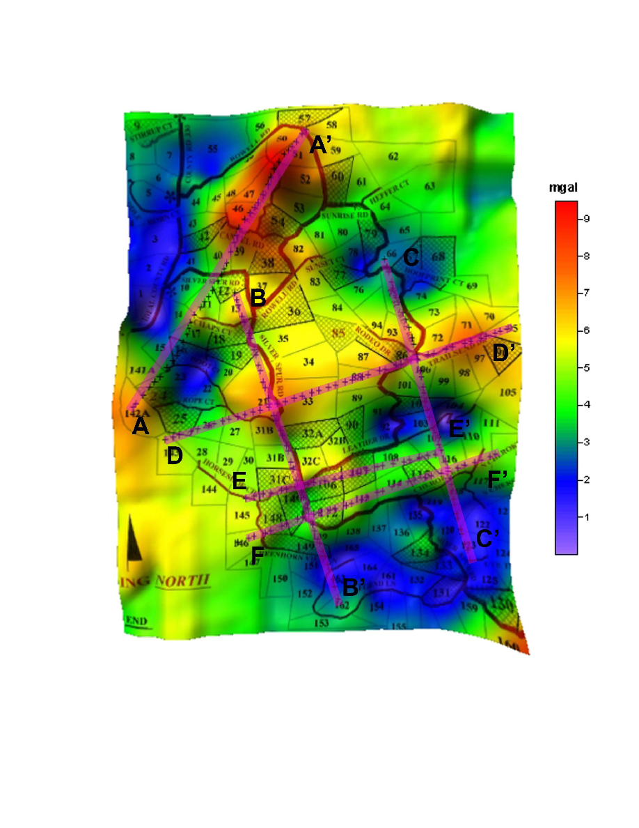
The complete Bouguer anomaly map with 6 selected 2.5D profiles lines is shown in Figure 18.
Four of the lines are taken along the trend of the gravity anomalies and two are taken
perpendicular. Gravity values are extracted along these profiles and block models are created to
match the gravity changes.
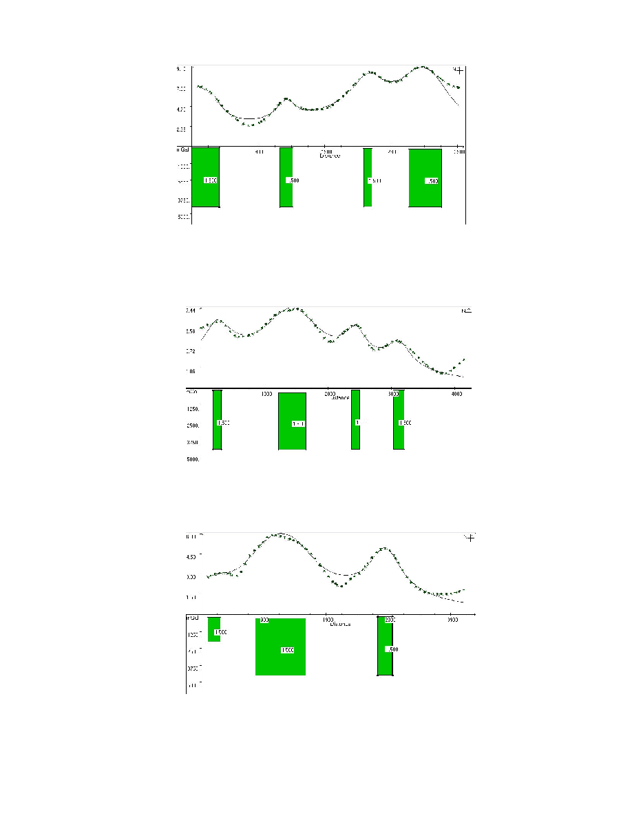
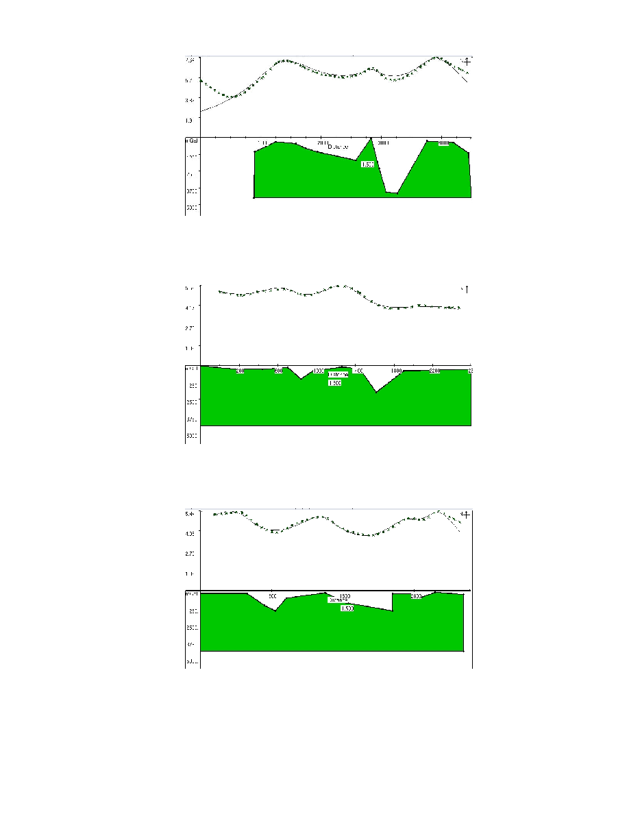
Profile AA' , Figure 19, is a 2D cross section which starts near the end of Rope Ct and trends
northeast to Reins Rd. The starred (*) points represent gravity values in mgals which have been
extracted from the complete Bouguer map along the AA' profile. The solid line is the gravity
computed for the model blocks shown in green. Depth and horizontal axis units are meters.
The object of gravity modeling is to match the computed gravity anomaly with the observed gravity
values. The resulting model reflects the depth and extent of dike structures.
A constant density is required for computing the gravity field. Values shown on the green blocks
represent density contrast values between the dike rock and the surrounding sandstone. Referring
to Table 1 for measured density values, a value of 1.5 was chosen to represent the density
contrast. This value was used for all density blocks for consistency. Surface positions and lateral
extent of the density blocks are shown in Figure 25.
The topographic map, Figure 16, suggests that ridges to the west of the survey may extend into the
The Ranch. Body 1 on Profile AA' indicates a dike extending along the trend of the ridge possibly
extending the length of Profile AA'. Body 2 is a cross cutting dike. It shows up again in Profile BB'
and extends the length of Rowell Rd to Sunset Ct. Body 3 required a long lateral extent to match
the gravity anomaly. The lateral extent may indicate a possible influence from the large gravity
anomaly related to Body 4. A dike outcrop in the creek bed along Silver Spur Rd indicates that the
dike associated with Body 3 most likely trends to the northwest. Body 4 has a large associated
gravity anomaly and may either be an extension of the dike from the south or an extension from a
dike trending west to east outside The Ranch or both. Depths to the top of the dikes vary from 80-
90m for dikes 1 and 2 along the south side to depths of 140-200m along Reins Rd to the north.
Figure 26 shows a possible interpretation of the cross cutting dike structure.
Profile BB', Figure 20, starts along Silver Spur Rd to the north and runs SSE to the south end of
The Ranch. As mentioned, Body 1 most likely extends along Rowell Rd to Sunset Ct and possibly
beyond. Body 2 is a broad gravity anomaly that ranges across The Ranch to at least Sunrise Rd.
A short lateral extent was used for the density block. The computed gravity anomaly was relatively
insensitive to lateral extent because of the required depth of the perturbing blocks. The dike
appears to start around Boot Ct and extends to Sunrise Rd. Body 3 indicates a cross cutting dike
structure that trends west to east along Horseshoe Ct and Leather Dr. The anomaly is discussed in
detail for Profile EE'. Similarly, Body 4 shows the intersection of Profile BB' with the Small Dike
anomaly along Profile FF'. Depths to top of the anomalies range from 110-140m for the narrow

7
cross cutting dikes, Bodies 3 and 4, to a relatively deep 325m for the broad anomaly associated
with Body 2.
Profile CC', Figure 21, follows Sunrise Rd and intersects Small Dike to the south. Body 1 may be a
small dike following the west to east trend shared with the major dike features. Body 2 is an
extension of the broad gravity anomaly seen along Profile BB'. The gravity anomaly appears
smeared and may indicate 3D effects from nearby features. Profile DD' along the ridge of the
broad dike feature shows a break in the anomaly at the intersection with Profile BB'. The break
may indicate a fault which strikes NNE and will be discussed in more detail when profiles DD' and
EE' are evaluated. Body 3 represents the intersection with Small Dike to the south. Bodies 1 and 3
are at depths of 200 m and 180 m respectively. Body 2 is modeled at a depth of 300 m and may
reflect a discontinuity along the west to east anomaly modeled in Profile DD'.
Profile DD', Figure 22, starts on the west at Boot Ct, traverses across Silver Spur Rd to Sunrise Rd
and ends along Trails End Dr to the east. The gravity anomaly is wide and may indicate a
contribution from a second dike within the anomaly. A single polygon is used to model the gravity
anomaly since the profile traverses along the ridge of the anomaly. The anomaly begins abruptly
around the start of Boot Ct. Profile DD' shows the top of dike gently dipping to the east, starting at
a depth of 315m and dropping to a depth of 1700m. A small anomaly along Rodeo Dr brings the
depth back to 30m near the surface. The depth plunges to 4000m and then returns to 250m
beneath Trails End Dr. The large depth variation may indicate the dike is offset by a fault. Further
evidence for a fault can be found along Profile EE'. The interpretation of the dike and fault are
shown in Figure 26.
Profile EE', Figure 23, starts along Horseshoe Circle to the west and travels along Leather Dr down
to the old Hezron Mine. The top of the interpreted dike varies from 200-300m along the profile until
about property 107 where the interpreted dike drops to a depth of 2000m then returns to a depth of
400m along the Hezron mine ridge. The drop along the top of the surface of the model is
interpreted as a fault in Figure 26.
Profile FF', Figure 24, starts along Green Horn View Lane, travels along Silver Spur Rd following
Small Dike and ends along Cherokee Lane to the east. The top of the model drops to a depth of
1500m where it first intersects Silver Spur Rd. This may indicate a fault or a smaller cross cutting
dike feature. The model returns to a depth of 140m before dropping again to 1500m. This second
drop is interpreted as an extension of the fault along Sunrise Rd and Leather Drive. The model
returns to a depth of 220m along Cherokee Lane.
Profiles BB' and CC' extend into what appears to be a broad, isolated basin between Small Dike
and Big Dike on the south end of The Ranch. A small gravity high occurs in the basin around
property 134, but the basin is featureless for the most part. Small gravity changes do not
necessarily translate into small topography changes. A surface elevation change of 70m along
Pryor Canyon is seen in the same area.
Water Regions
Dikes form impermeable boundaries to water flow. Knowing the position of the dikes, possible
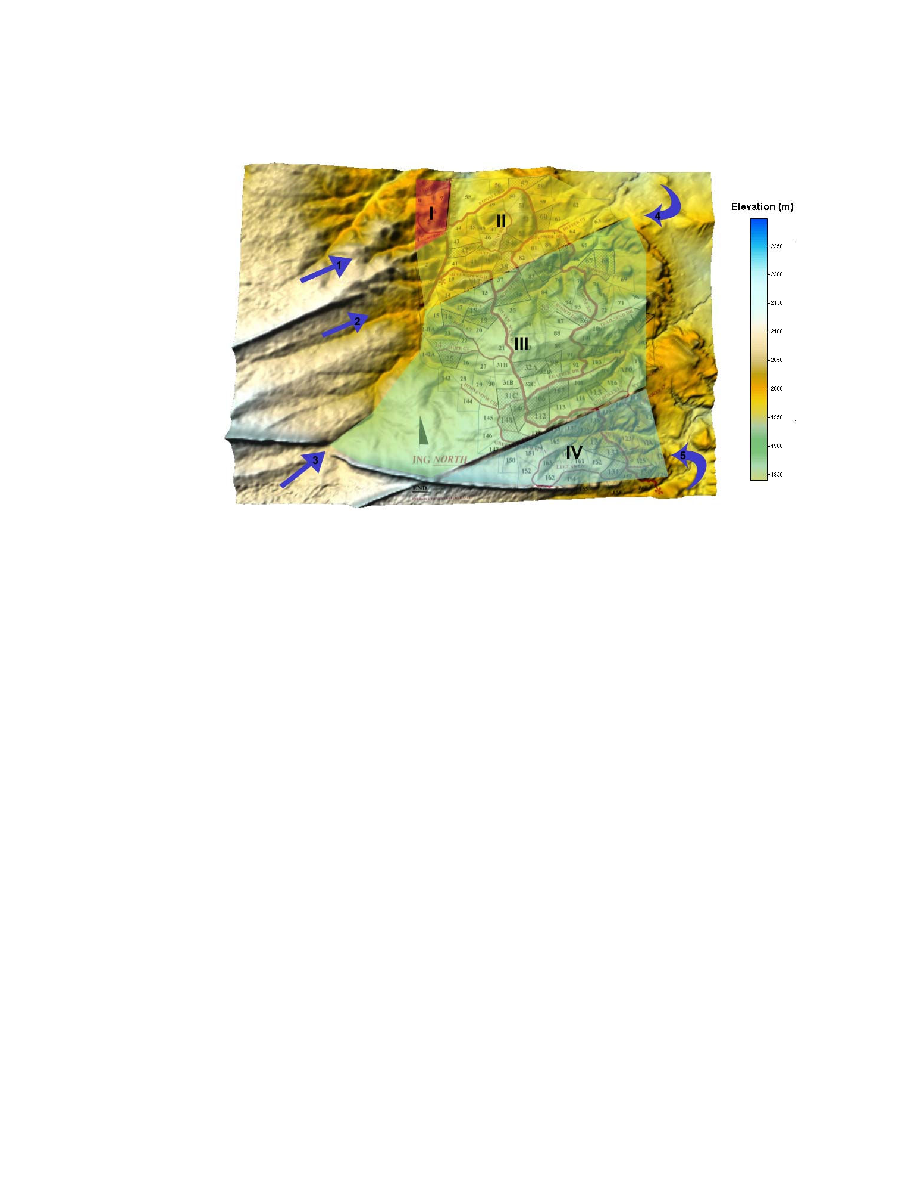
water flow regions can be inferred. Figure 27 shows five possible recharge regions associated with
the interpreted dike positions. Recharge areas are marked with blue arrows. Any changes to
recharge regions in the blue arrow areas may impact well performance in the associated regions on
The Ranch.
Region I in the northwest corner of The Ranch was not included in the gravity survey but from the
topographic expression of dikes to the west, it is reasonable to assume that water recharge occurs
along the dike to the immediate south and is replenished with any available water resource coming
from the northwest. The recharge area is marked with blue arrow 1.

8
Region II at the north end of the Ranch receives recharge water from the south side of the dike to
the immediate west. The recharge area is marked with blue arrow 2. The interpreted dike along
Reins Rd may redirect the recharge coming from the west causing shadow zones on the east side
of the dike. An alternate recharge region to the northeast is marked with blue arrow 4.
Region III in the center of The Ranch has a possible recharge area occurring along Walsen Creek.
The digital elevation map, Figure 27, shows a large fault offsetting Big Dike along Walsen Creek as
indicated with blue arrow 3. The fault offset creates a gap of 100m allowing water recharge to flow
off the slopes of East Spanish Peak and enter the Region III water regime from the south. The
interpreted dike which begins along Chaps Ct and extends along Rowell Rd to Sunrise Ct may
discourage recharge from entering Region II from this recharge source. Small Dike bounds Region
III on the south. Seasonal recharge occurs along the flanks of Small Dike. Along the northeast
margin of Region III recharge marked as blue arrow 4 may occur from the plains to the northeast.
Region IV at the south end of The Ranch is isolated from the other recharge zones by Small Dike
and Big Dike. The gravity survey indicates that the region is an isolated basin. Figure 5 shows
Pryor Canyon beginning along the west edge of Small Dike. Surface runoff travels down Pryor
Canyon seeping into fractures along the surface and recharging water resources at depth. A
similar type of recharge mechanism occurs along the north side of Big Dike. Water recharge
marked as blue arrow 5 may also occur on the southeast margin.
Depths to the top of dike structures are greater than 100m in most areas on The Ranch. This
means deep water flow is influenced by dike positions, but near the surface water flow is controlled
by existing fractures. Figure 3 shows vertical fractures occurring in the Trinidad sandstone. Similar
fractures most likely exist in the Raton sandstone that covers most of The Ranch.
Summary
Gravity surveys are a relatively inexpensive geophysical method which can be used to infer simple
subsurface features. The intruded dike complex which permeates Silver Spur Ranch provides a
density contrast signature which is measurable. The impermeable dikes impact water flow in the
region. By knowing the location of subsurface dikes, possible water flow regions are inferred.
The final interpretation, Figure 26, shows dike and fault positions interpreted from the gravity
survey. Long linear ridges to the west are consistent with interpreted dikes on The Ranch. Dike
ridges tend to lose their distinct appearance once they cross Walsen Arroyo into the Ranch. The
gravity survey confirms that the dikes extend into The Ranch at depth.
The gravity anomaly along Reins Rd may represent an extension of a dike from the south west. A
dike outcrop in Walsen Arroyo supports this interpretation. The small SSW to NNE trending
anomaly which starts at Chaps Ct, crosses Cantrell Rd and continues along Reins Rd, does not
correlate well with the predominate dike orientations in the area. However, a dike outcrop along
Silver Spur Rd is consistent with the interpretation.
Southwest to northeast trending gravity anomalies correlate well with dikes to the west. Big Dike
and Small Dike show positive gravity anomalies. There are 3 smaller east-west trends which
indicate buried dikes with depths that range from a hundred meters to thousands of meters.
Along Sunrise Rd the interpreted east-west dike structures drops thousands of meters. This is
interpreted as a possible fault which offsets the dike. A large drop in interpreted depth to the top of
the structure along Leather Dr and Silver Spurs Rd to south may be an extension of the same fault.

9
The region south of Small Dike and north of Big Dike on the south end of The Ranch is relatively
free of gravity anomalies. This indicates a large basin with water recharge coming from the
bounding Big Dike and Small Dike ridges.
Water regions are defined based on dike locations, Figure 27. There are at least four separate
water regions with corresponding recharge areas. Dikes permeate the subsurface at depths of
more than 100m. This means the dikes control water flow at depth, but near the surface water is
controlled by fractures in the overburden.
Future Studies
The gravity survey successfully delineated the general structure of the subsurface dikes. These
dikes are a controlling influence on water flow at depth. Above the dikes, water flow is controlled by
fractures in the sedimentary rock. Fractures most likely follow the vertical fracture patterns created
during the emplacement of the dikes.
For water wells, it is important to know if and where there are fluid filled fractures. One geophysical
method that is sensitive to vertical water filled fractures is a method called resistivity. Resistivity
surveys measure the electrical conductivity of the earth. A small electrical current is applied to the
earth through a pair of electrodes. Another pair of electrodes is used to measure the variation in
the electrical field away from the source electrodes. The small current created by 4 D size batteries
is non-destructive and does not harm vegetation or structures. A useful study would be to
determine the sensitivity of this type of survey in the area.
A near surface seismic survey is more expensive but gives more detail about near surface layers
and fracturing. Seismic surveys use a shotgun source which is shot into the ground to generate
sound waves. Sound waves are reflected at rock layer boundaries or faults and return to the
surface. An array of accelerometers is set on the surface of the earth to record the returning sound
waves. Records are processed to create seismic sections which show rock interfaces at depth.
The sections outline in detail the existing fracture patterns, but do not guarantee water filled
fractures.
Finally, the most accurate measure of the subsurface comes from well data. This is the only direct
measurements of the subsurface. Well monitoring will establish seasonal norms for existing wells.
A sharp drop or increase from the norm indicates a change in water recharge patterns or water
supply. A useful study would be to establish monitoring wells which can be measured monthly. To
give a good measurement of static water levels, the monitor well should not be one that is currently
being pumped.
10
Figure 1 Radial dike outcrop along Highway of Legends north of La Veta.
Figure 2 Aerial photo of Spanish Peaks looking west from Silver Spurs Ranch. Major radial dike
locations are outlined in blue.
11
Figure 3 Vertical fractures in the Trinidad sandstone found along County Rd 330 between The
Ranch and Walsenburg.
Figure 4 Gravity station locations in yellow and rock sample locations in white. Big Dike and Small
Dike can be seen extending into The Ranch.
12
Figure 5 USGS topographic map showing gravity station locations in blue. Road locations appear
as they were in the early `90s. Gravity station locations indicate position of current roads.
13
Figure 6 Silver Spurs Ranch property map as of July 2005. The map is used for reference on the
gravity anomaly maps.
Figure 7 Mosaic of digital elevation maps for the area with property map.
14
Figure 8 Typical gravity station measurement showing the gravity meter, GPS receiver and field
notebook. The towel is for an old man's knees.
Figure 9 Top view of LaCoste and Romberg D gravity meter. Tilt adjustment knobs are located
on the left and middle right. Galvanometer dial is above the eyepiece and the aluminum
read out dial is in the middle.
15
Figure 10 Schematic showing a cross section of the gravity meter. The ultra sensitive Zero Length
Spring balances the Mass on the balance Beam. The galvanometer `beam' measures the
Long Lever location with respect to zero.
Figure 11 Elevation profile along Silver Spur Rd starting at the mail boxes on the County Rd 330
and ending at the south entrance. Yellow line shows gravity datum elevation at 2076m.
Vertical exaggeration is a factor of 12.
16
Figure 12 Free air anomaly map shown with regional topography. Red gravity anomaly contours
trend along surface ridges.
Figure 13 Free air anomaly map shown with property map.
17
Figure 14 Bouguer anomaly map shown with regional topography.
Figure 15 Bouguer anomaly map with property map.
18
Figure 16 Complete Bouguer anomaly map shown with regional topography.
Figure 17 Complete Bouguer anomaly map with property map.
19
Figure 18 Complete Bouguer anomaly map with gravity modeling profiles.
20
Figure 19 Profile AA', Rope Ct to Reins Rd.
Figure 20 Profile BB', north end of Silver Spurs Rd.
Figure 21 Profile CC', Sunrise Rd to south Silver Spurs Rd.
21
Figure 22 Profile DD', Rope Ct to Trails End Dr.
Figure 23 Profile EE', Horseshoe Ct to Leather Dr.
Figure 24 Profile FF', Green Horn View Ln to Cherokee Ln.
22
Figure 25 Lateral position of constant density gravity blocks marked in green.
Figure 26 Final interpretations of dike locations. NNE trending fault in cyan is shown extending
from Sunrise Rd to Leather Dr.
23
Figure 27 Water regions with recharge areas marked with blue arrows.

24
Appendix A
Gravity correction formulas
Drift correction:
g
dc
= g
obs
[(g
base2
-
g
base1
)/(t
base2
t
base1
)]X(t
obs
t
base1
)
g
obs
= observed gravity
g
base
= gravity at base station
t
obs
= time of gravity observation
t
base
= time of observation at base station
Latitude correction:
g
IGF
= 9.78032[(1 + 0.00193185138sin
2
)/(1 - .006694379sin
2
)
1/2
]
= geographic latitude in radians
Free air correction:
g
FA
= 0.3086*(surface elevation datum elevation) elevation in meters
Bouguer correction:
g
B
= g
FA
- 0.04193*density*(surface elevation datum elevation)
for an average density of 2.67 g/cc
g
B
= g
FA
- 0.112*( surface elevation datum elevation)
g
B
= 0.1966*(surface elevation datum elevation) elevation in
meters
Complete Bouger correction:
g
CB
= g
dc
g
IGF
+ g
B
+ terrain correction

25
Appendix B
Table 2 Gravity measurements and corrections.
Gravity units are in mgal. UTM XY locations and elevations are in meters.
stn
x
y
elev
field g
rel g
latitude
free air
bouguer
complete
B1
522518
4152400
2076
913.10
106.15
106.15
106.15
106.15
111.82
1
522501
4152445
2075
917.76
106.71
106.68
106.37
106.48
111.56
2
522603
4152467
2069
924.49
107.54
107.48
105.32
106.11
110.48
3
522703
4152480
2065
927.15
107.86
107.80
104.41
105.64
109.81
4
522806
4152490
2060
933.81
108.65
108.59
103.65
105.44
109.64
5
522905
4152503
2060
935.13
108.86
108.78
103.84
105.63
109.57
6
522998
4152533
2057
941.69
109.65
109.54
103.68
105.81
109.41
7
523092
4152572
2053
952.82
110.98
110.84
103.74
106.32
109.84
8
523186
4152602
2051
960.67
111.83
111.67
103.96
106.76
110.05
9
523280
4152639
2049
962.05
111.97
111.78
103.45
106.47
109.12
10
523373
4152678
2042
969.12
112.77
112.55
102.06
105.86
108.30
11
523457
4152730
2039
976.83
113.64
113.38
101.96
106.11
109.01
12
523546
4152775
2040
987.61
114.87
114.58
103.47
107.50
109.80
13
523639
4152816
2036
985.36
114.59
114.27
101.92
106.40
108.03
14
523720
4152875
2028
997.12
115.94
115.57
100.76
106.13
106.58
15
523786
4152916
2015
1005.54
116.90
116.49
97.67
104.50
104.78
16
523752
4152827
2013
1016.13
118.11
117.78
98.34
105.39
105.56
17
523832
4152855
2005
1038.55
120.69
120.34
98.43
106.38
106.74
18
523916
4152903
1999
1050.88
122.11
121.71
97.95
106.57
107.23
19
523976
4152989
1993
1062.21
123.40
122.94
97.33
106.62
107.25
20
524000
4153076
1992
1073.76
124.73
124.20
98.28
107.68
110.99
21
523056
4152638
2049
963.36
111.84
111.65
103.32
106.34
108.80
22
523078
4152738
2039
975.30
113.22
112.95
101.53
105.68
107.28
23
523150
4152801
2029
993.36
115.31
115.00
100.49
105.75
107.38
24
523097
4152873
2028
1005.85
116.75
116.38
101.57
106.94
107.70
25
523017
4152921
2017
1017.21
118.07
117.66
99.45
106.05
107.71
26
522990
4153015
2026
1008.03
116.98
116.49
101.06
106.66
109.52
27
523049
4153095
2034
1000.71
116.12
115.57
102.61
107.31
110.52
28
523089
4153173
2039
991.64
115.05
114.45
103.03
107.17
111.09
29
523007
4153234
2045
977.50
113.40
112.75
103.18
106.65
111.38
30
522920
4153281
2052
973.68
112.60
111.91
104.50
107.19
112.46
31
522847
4153346
2056
967.56
111.92
111.18
105.00
107.24
112.83
32
522829
4153424
2061
956.99
110.72
109.92
105.29
106.97
113.25
33
522884
4153514
2066
952.55
110.23
109.36
106.27
107.39
114.31
34
522970
4153557
2068
950.34
110.00
109.09
106.62
107.51
114.19
35
523062
4153598
2065
950.66
110.06
109.12
105.72
106.96
113.04
36
523151
4153650
2062
957.13
110.83
109.85
105.53
107.10
112.88
37
523230
4153772
2057
966.48
111.65
110.57
104.71
106.84
113.51
38
523146
4153831
2061
963.71
111.54
110.41
105.79
107.46
114.25
39
523063
4153894
2061
971.36
112.40
111.22
106.59
108.27
114.55
40
522975
4153931
2059
974.51
112.73
111.53
106.28
108.18
114.63
41
522871
4153945
2057
975.50
112.80
111.59
105.72
107.85
114.16
42
522782
4153982
2055
978.42
113.12
111.87
105.39
107.74
113.79

26
stn
x
y
elev
field g
rel g
latitude
free air
bouguer
complete
43
522688
4154074
2051
990.52
114.49
113.17
105.46
108.26
114.10
44
523330
4153737
2055
973.72
112.51
111.45
104.97
107.32
113.16
45
523429
4153732
2055
976.64
112.84
111.79
105.31
107.66
113.56
46
523524
4153766
2055
980.32
113.26
112.19
105.71
108.06
113.56
47
523605
4153821
2057
980.95
113.33
112.22
106.35
108.48
114.47
48
523693
4153870
2054
983.60
113.64
112.48
105.69
108.16
114.52
49
523788
4153892
2057
982.16
113.47
112.30
106.43
108.56
115.17
50
523883
4153920
2059
978.85
113.08
111.89
106.64
108.54
115.70
51
524007
4153978
2063
975.26
112.66
111.42
107.41
108.86
115.03
52
523285
4153856
2056
971.09
112.12
110.97
104.80
107.04
113.03
53
523325
4153950
2056
976.93
112.73
111.51
105.34
107.58
113.70
54
523325
4154050
2052
984.91
113.61
112.32
104.91
107.60
113.63
55
523254
4154124
2050
992.28
114.42
113.07
105.04
107.95
113.71
56
523190
4154207
2046
1001.95
115.49
114.06
104.81
108.16
112.89
57
523156
4154299
2038
1020.28
117.55
116.06
104.33
108.59
112.97
58
523119
4154391
2030
1039.73
119.75
118.19
103.99
109.14
112.56
59
523104
4154499
2019
1050.13
120.90
119.25
101.66
108.04
111.08
60
523149
4154578
2014
1057.98
121.76
120.04
100.91
107.85
110.29
61
523235
4154638
2007
1075.24
123.72
121.96
100.66
108.39
110.54
62
523293
4154714
2000
1090.13
125.40
123.58
100.13
108.64
110.42
63
523399
4154718
1999
1095.85
126.01
124.19
100.43
109.05
110.75
64
523485
4154674
1996
1095.44
125.91
124.12
99.43
108.39
109.63
65
523562
4154587
1995
1100.50
126.46
124.74
99.74
108.81
111.61
66
523123
4154685
2013
1067.29
122.50
120.71
101.26
108.32
111.48
67
523106
4154780
2012
1076.97
123.57
121.70
101.95
109.12
111.46
68
523021
4154837
2003
1097.94
125.95
124.03
101.50
109.67
111.41
69
522938
4154894
1996
1109.33
127.27
125.31
100.62
109.57
111.57
70
522847
4154873
1999
1110.72
127.43
125.48
101.72
110.34
112.18
71
522753
4154827
1998
1105.29
126.80
124.89
100.82
109.55
111.03
72
522666
4154838
1994
1105.29
126.80
124.88
99.57
108.75
110.16
73
522651
4154928
1992
1104.80
126.74
124.75
98.82
108.23
109.81
74
522724
4154999
1993
1107.83
127.34
125.29
99.68
108.97
110.63
75
522787
4155075
1990
1108.04
127.36
125.25
98.71
108.34
110.52
76
522819
4155167
1997
1110.58
127.65
125.47
101.09
109.93
112.37
77
522897
4155225
1996
1109.29
127.49
125.27
100.58
109.53
111.51
78
522891
4155317
1993
1115.88
128.25
125.95
100.34
109.63
111.29
80
522764
4155469
1991
1123.85
129.17
126.75
100.52
110.04
112.49
81
522721
4155563
1995
1123.65
129.14
126.65
101.65
110.72
112.68
79
522845
4155402
1992
1121.27
128.85
126.49
100.57
109.97
112.32
82
522659
4155638
1993
1128.18
129.65
127.10
101.48
110.78
112.88
83
522575
4155681
1990
1136.13
130.56
127.98
101.44
111.07
112.57
84
522616
4155758
1984
1147.90
131.92
129.28
100.89
111.19
112.59
85
522707
4155807
1981
1155.94
132.85
130.17
100.85
111.49
112.78
86
522803
4155866
1979
1161.76
133.52
130.79
100.86
111.72
113.64
87
522460
4155691
1988
1136.46
130.57
127.98
100.82
110.67
112.78
88
522360
4155686
1990
1132.73
130.13
127.54
101.00
110.63
112.82
89
522262
4155670
1991
1130.68
129.88
127.31
101.08
110.59
113.58

27
stn
x
y
elev
field g
rel g
latitude
free air
bouguer
complete
90
522131
4155670
1999
1117.25
128.31
125.74
101.97
110.59
113.81
91
522142
4155772
2000
1118.02
128.37
125.72
102.26
110.77
114.65
92
522123
4155874
2005
1115.08
128.02
125.29
103.38
111.32
115.85
93
522093
4155970
2010
1105.46
126.90
124.09
103.72
111.11
115.77
94
522066
4156055
2010
1100.80
126.35
123.47
103.10
110.49
114.96
95
522042
4156151
2007
1109.04
127.30
124.35
103.05
110.78
115.34
96
522016
4156250
2010
1100.68
126.32
123.29
102.92
110.31
115.32
97
521989
4156345
2010
1098.83
126.10
122.99
102.62
110.01
115.12
98
521927
4156433
2010
1100.97
126.34
123.17
102.80
110.19
115.60
99
521860
4156507
2012
1108.65
127.23
123.99
104.24
111.41
115.77
100
521775
4156561
2004
1114.43
127.89
124.62
102.40
110.46
114.26
101
521681
4156590
1999
1120.22
128.56
125.26
101.50
110.12
114.24
102
521588
4156573
1999
1129.98
129.69
126.40
102.64
111.26
114.68
103
521512
4156510
1993
1144.28
131.34
128.10
102.49
111.78
114.22
104
521420
4156456
1987
1151.66
132.19
129.00
101.53
111.49
113.72
105
521326
4156411
1981
1157.23
132.84
129.68
100.37
111.00
112.84
106
521235
4156376
1976
1158.92
133.04
129.91
99.05
110.25
111.45
107
521140
4156344
1972
1160.67
133.25
130.14
98.05
109.69
110.79
108
521045
4156309
1971
1166.16
133.89
130.81
98.41
110.16
110.98
109
520969
4156244
1971
1162.23
133.44
130.41
98.01
109.76
110.44
110
520884
4156187
1967
1178.76
135.37
132.38
98.75
110.95
111.14
111
520794
4156144
1959
1180.77
135.60
132.65
96.55
109.64
109.79
112
520692
4156136
1955
1182.74
135.84
132.89
95.55
109.10
109.23
113
520610
4156075
1957
1183.97
135.98
133.09
96.36
109.68
109.83
114
520535
4156010
1957
1189.74
136.66
133.81
97.09
110.41
110.85
115
520443
4155977
1950
1202.01
138.09
135.27
96.38
110.49
110.91
116
520360
4155923
1951
1191.48
136.87
134.09
95.51
109.51
109.62
117
520279
4155943
1960
1179.03
135.42
132.63
96.83
109.82
112.96
118
522037
4155555
1999
1109.63
127.40
124.92
101.16
109.78
112.64
119
521944
4155492
2000
1103.66
126.72
124.29
100.83
109.34
112.43
120
521862
4155429
2003
1099.33
126.23
123.84
101.31
109.49
112.77
121
521805
4155346
2009
1089.06
125.04
122.72
102.04
109.55
113.58
122
521739
4155268
2014
1073.88
123.29
121.03
101.90
108.84
113.65
123
521664
4155223
2022
1060.48
121.74
119.52
102.85
108.90
113.94
124
521541
4155238
2024
1065.32
122.31
120.08
104.03
109.85
115.68
125
521438
4155193
2032
1053.14
120.91
118.71
105.13
110.05
116.46
126
521351
4155221
2037
1042.76
119.71
117.49
105.46
109.82
116.66
127
521348
4155313
2040
1038.06
119.18
116.88
105.77
109.80
116.76
128
521364
4155409
2040
1030.20
118.27
115.90
104.79
108.82
115.81
129
521408
4155513
2039
1030.62
118.33
115.88
104.46
108.60
115.60
130
521462
4155604
2038
1031.67
118.46
115.94
104.21
108.46
115.48
131
521509
4155694
2037
1035.18
118.88
116.28
104.25
108.61
116.05
132
521574
4155770
2040
1035.60
118.93
116.28
105.17
109.20
116.99
133
521600
4155870
2042
1032.89
118.63
115.90
105.40
109.21
117.46
134
521569
4155966
2045
1036.47
119.06
116.25
106.68
110.15
118.42
135
521499
4156044
2044
1037.74
119.22
116.35
106.48
110.06
117.75
136
521443
4156129
2041
1045.04
120.07
117.13
106.33
110.25
117.20

28
stn
x
y
elev
field g
rel g
latitude
free air
bouguer
complete
137
521231
4155233
2042
1035.18
118.93
116.70
106.20
110.01
116.56
138
521144
4155285
2041
1037.79
119.23
116.96
106.16
110.08
117.15
139
521043
4155329
2042
1033.88
118.78
116.47
105.98
109.79
116.56
140
520993
4155429
2038
1043.28
119.88
117.49
105.76
110.02
116.47
141
520961
4155512
2034
1043.67
119.92
117.47
104.51
109.21
115.13
142
521618
4155101
2034
1031.88
118.56
116.43
103.47
108.17
115.02
143
521599
4155011
2044
1017.24
116.86
114.80
104.92
108.51
115.77
144
521666
4154931
2049
1008.66
115.86
113.87
105.53
108.56
115.62
145
521726
4154852
2048
1009.29
115.94
114.00
105.36
108.50
115.04
146
521743
4154795
2044
1010.90
116.12
114.24
104.36
107.95
114.02
147
521831
4154867
2042
1018.30
116.99
115.04
104.55
108.36
114.88
148
521916
4154934
2042
1018.49
117.01
115.01
104.52
108.33
114.93
149
522009
4154984
2042
1017.60
116.91
114.87
104.38
108.19
115.14
150
521678
4154719
2049
1008.91
115.90
114.07
105.74
108.76
115.29
151
521609
4154646
2046
1009.23
115.94
114.17
104.91
108.27
114.59
152
521536
4154576
2042
1009.95
116.03
114.31
103.82
107.62
113.47
153
521468
4154500
2042
1017.22
116.87
115.22
104.73
108.53
114.47
154
521392
4154433
2044
1010.84
116.13
114.53
104.65
108.24
113.91
155
521249
4154370
2046
1002.21
115.13
113.58
104.32
107.68
113.23
156
521209
4154473
2043
1021.91
117.38
115.74
105.56
109.25
114.48
157
521190
4154573
2035
1038.27
119.27
117.55
104.90
109.49
114.25
158
521182
4154678
2029
1044.54
119.98
118.19
103.68
108.94
113.36
159
521170
4154791
2024
1062.05
122.01
120.12
104.07
109.89
113.74
160
521077
4154830
2018
1071.43
123.08
121.17
103.27
109.76
113.09
161
520977
4154831
2013
1090.12
125.24
123.33
103.88
110.94
113.75
162
520874
4154822
2007
1095.90
125.90
123.99
102.70
110.42
112.44
163
520777
4154827
2000
1107.31
127.22
125.30
101.85
110.36
111.91
164
520663
4154829
1995
1116.02
128.21
126.30
101.30
110.37
111.53
165
520572
4154869
1990
1124.10
129.14
127.20
100.66
110.28
111.01
166
520482
4154913
1984
1134.21
130.30
128.32
99.93
110.23
110.38
167
520367
4154950
1973
1143.90
131.41
129.40
97.61
109.14
109.37
168
520272
4154891
1976
1146.40
131.68
129.72
98.86
110.05
110.18
169
520183
4154835
1972
1145.06
131.52
129.59
97.50
109.14
109.30
170
520027
4154750
1976
1138.61
130.75
128.89
98.03
109.23
109.37
171
520312
4156849
1950
1208.63
138.85
135.34
96.46
110.56
110.76
172
520314
4156744
1946
1211.01
139.12
135.70
95.58
110.13
110.27
173
520314
4156638
1949
1209.75
138.97
135.63
96.44
110.65
110.78
174
520312
4156538
1951
1199.17
137.74
134.47
95.90
109.89
110.03
175
520309
4156429
1952
1192.18
136.92
133.74
95.47
109.36
109.48
176
520306
4156333
1955
1185.16
136.10
133.00
95.66
109.20
109.38
177
520305
4156228
1957
1183.38
135.89
132.87
96.15
109.47
109.61
178
520298
4156128
1955
1184.38
136.00
133.06
95.72
109.27
109.42
179
520282
4156020
1959
1183.20
135.86
133.00
96.90
110.00
110.11
180
520262
4155917
1960
1178.09
135.26
132.49
96.69
109.68
109.83
181
520241
4155813
1958
1177.08
135.14
132.45
96.03
109.24
109.50
182
520230
4155712
1957
1175.63
134.97
132.36
95.63
108.95
109.22
183
520239
4155601
1958
1173.25
134.69
132.16
95.75
108.96
109.11

29
stn
x
y
elev
field g
rel g
latitude
free air
bouguer
complete
184
520249
4155506
1962
1163.70
133.57
131.12
95.94
108.71
108.87
185
520254
4155408
1963
1163.16
133.51
131.13
96.26
108.91
109.05
186
520254
4155307
1965
1160.50
133.19
130.90
96.65
109.07
109.22
187
520219
4155210
1966
1154.95
132.55
130.33
96.38
108.70
108.85
188
520189
4155116
1967
1147.46
131.67
129.53
95.89
108.09
108.23
189
520155
4155016
1973
1144.47
131.32
129.26
97.47
109.00
109.16
190
520099
4154927
1975
1140.92
130.91
128.92
97.75
109.05
109.28
191
520051
4154835
1976
1138.35
130.61
128.69
97.83
109.03
109.20
192
520010
4154729
1977
1134.24
130.14
128.30
97.75
108.83
109.22
193
519970
4154629
1983
1125.51
129.13
127.37
98.67
109.08
109.41
194
519915
4154542
1982
1117.42
128.19
126.50
97.49
108.01
108.18
195
519869
4154451
1981
1117.73
128.22
126.60
97.29
107.92
108.12
196
519837
4154344
1978
1113.25
127.71
126.17
95.93
106.90
107.03
197
519789
4154250
1984
1102.36
126.44
124.98
96.59
106.89
107.57
198
519680
4154181
1995
1087.42
124.71
123.30
98.30
107.37
108.30
199
519583
4154135
1999
1078.03
123.62
122.25
98.49
107.11
113.51
200
521263
4154274
2051
993.31
113.78
112.30
104.58
107.38
114.61
201
521165
4154236
2056
986.35
112.97
111.52
105.35
107.59
114.49
202
521068
4154192
2057
992.82
113.72
112.31
106.45
108.57
114.81
203
520970
4154186
2051
997.29
114.25
112.84
105.12
107.92
113.81
204
520868
4154221
2047
1002.26
114.83
113.39
104.44
107.69
113.36
205
520771
4154265
2041
1008.17
115.52
114.04
103.24
107.16
112.40
206
520672
4154278
2040
1013.04
116.09
114.61
103.50
107.53
112.37
207
520597
4154224
2037
1027.73
117.80
116.36
104.33
108.69
114.80
208
521255
4154168
2050
997.08
114.24
112.85
104.82
107.73
113.76
209
521228
4154068
2051
989.42
113.35
112.04
104.32
107.12
112.86
210
521213
4153968
2050
988.68
113.27
112.03
104.01
106.92
112.75
211
521315
4153902
2052
982.91
112.60
111.42
104.01
106.70
113.15
212
521370
4153815
2056
974.67
111.65
110.53
104.36
106.60
112.96
213
521426
4153732
2060
968.86
110.98
109.92
104.99
106.78
113.30
214
521475
4153644
2063
960.80
110.04
109.06
105.05
106.51
113.63
215
521502
4153548
2070
952.16
109.04
108.14
106.28
106.96
114.12
216
521509
4153446
2072
945.26
108.24
107.42
106.18
106.63
114.68
217
521493
4153341
2082
934.35
106.98
106.23
108.09
107.41
115.41
218
521529
4153252
2083
924.88
105.85
105.18
107.34
106.55
114.75
219
521603
4153180
2086
919.33
105.20
104.58
107.67
106.55
115.25
220
521624
4153075
2089
917.42
104.98
104.44
108.46
107.00
114.93
221
521574
4152945
2084
923.30
105.66
105.23
107.69
106.80
114.37
222
521474
4152980
2087
928.51
106.26
105.80
109.20
107.96
115.40
223
521366
4152996
2082
938.42
107.41
106.94
108.79
108.12
114.82
224
521267
4152959
2076
946.51
108.35
107.90
107.90
107.90
113.85
225
521164
4152953
2069
953.65
109.18
108.74
106.58
107.36
113.35
226
521057
4153029
2068
956.43
109.50
109.01
106.54
107.43
113.35
227
520962
4153114
2066
961.26
110.07
109.50
106.42
107.54
113.74
228
520934
4153221
2067
967.67
110.82
110.17
107.39
108.40
114.54
229
520901
4153309
2065
972.72
111.41
110.69
107.29
108.52
114.05
230
520845
4153400
2061
969.83
111.07
110.28
105.66
107.33
112.53

30
stn
x
y
elev
field g
rel g
latitude
free air
bouguer
complete
231
520738
4153437
2054
970.36
111.14
110.32
103.53
105.99
110.42
232
520662
4153472
2046
994.13
113.91
113.06
103.80
107.16
110.02
233
520611
4153584
2029
1013.64
116.18
115.24
100.74
106.00
108.35
234
520518
4153643
2023
1026.25
117.65
116.66
100.31
106.24
108.76
235
520423
4153687
2024
1029.52
118.03
117.01
100.96
106.79
109.87
236
520270
4153718
2029
1018.45
116.75
115.70
101.20
106.46
110.30
237
520152
4153681
2037
1005.35
115.23
114.21
102.18
106.54
110.52
238
520116
4153638
2039
996.25
114.17
113.19
101.77
105.91
111.35
239
520831
4153150
2061
961.18
110.10
109.51
104.88
106.56
111.63
240
520722
4153115
2058
970.32
111.17
110.61
105.05
107.07
111.48
241
520606
4153102
2055
974.95
111.71
111.15
104.67
107.03
110.98
243
520398
4153147
2047
981.36
112.46
111.86
102.91
106.16
110.60
242
520504
4153127
2052
984.55
112.83
112.25
104.84
107.53
111.34
244
520311
4153182
2045
988.71
113.31
112.69
103.12
106.59
110.34
245
520198
4153212
2044
999.79
114.60
113.96
104.08
107.66
110.64
246
520061
4153176
2037
1009.75
115.76
115.14
103.11
107.47
115.08
247
521608
4152825
2083
925.98
106.02
105.68
107.84
107.06
113.59
248
521660
4152733
2078
927.94
106.25
105.98
106.60
106.38
112.53
249
521709
4152635
2076
919.02
105.21
105.02
105.02
105.02
111.16
250
521771
4152517
2078
916.44
104.91
104.82
105.44
105.21
111.49
251
521803
4152422
2081
914.83
104.73
104.71
106.25
105.69
112.16
252
521845
4152304
2085
909.61
104.12
104.19
106.97
105.96
112.65
253
521876
4152201
2089
903.87
103.45
103.61
107.62
106.16
112.85
254
521887
4152145
2090
903.17
103.37
103.57
107.89
106.32
112.82
255
521782
4152102
2089
900.20
103.02
103.26
107.27
105.81
112.49
256
521658
4152087
2091
889.13
101.74
101.98
106.61
104.93
111.98
257
521575
4152059
2095
886.72
101.46
101.72
107.59
105.46
112.38
258
521473
4151998
2095
887.16
101.51
101.82
107.69
105.56
111.72
259
521360
4151955
2092
887.76
101.58
101.93
106.86
105.07
111.90
260
521381
4151844
2097
879.73
100.64
101.08
107.56
105.21
112.04
261
521357
4151739
2099
882.13
100.92
101.44
108.54
105.96
112.47
262
521378
4151639
2098
879.12
100.57
101.17
107.96
105.50
111.90
263
521413
4151506
2103
867.50
99.22
99.92
108.26
105.23
112.26
264
521461
4151373
2108
853.25
97.56
98.37
108.25
104.66
111.22
265
521594
4151327
2108
848.01
96.96
97.80
107.67
104.09
109.78
266
522403
4152396
2076
927.71
106.14
106.14
106.14
106.14
112.18
267
522312
4152355
2080
918.91
105.11
105.15
106.38
105.93
112.23
268
522215
4152327
2083
911.05
104.19
104.25
106.41
105.62
112.03
269
522131
4152268
2085
902.44
103.18
103.29
106.06
105.06
111.85
270
522035
4152197
2090
896.00
102.42
102.58
106.90
105.34
111.54
271
521957
4152134
2089
902.11
103.13
103.34
107.35
105.89
111.60
272
521902
4152025
2083
907.54
103.75
104.05
106.21
105.42
110.05
273
521921
4151923
2078
913.85
104.48
104.86
105.47
105.25
109.50
274
521908
4151831
2073
924.21
105.68
106.13
105.20
105.54
109.86
275
521933
4151711
2076
919.71
105.15
105.69
105.69
105.69
109.99
276
522041
4151654
2080
908.58
103.85
104.44
105.67
105.22
110.58
277
522152
4151593
2088
896.64
102.46
103.09
106.79
105.45
110.76

31
stn
x
y
elev
field g
rel g
latitude
free air
bouguer
complete
278
522265
4151567
2088
889.57
101.63
102.28
105.99
104.64
109.78
279
522353
4151625
2082
903.83
103.28
103.89
105.74
105.07
109.98
280
522456
4151684
2082
908.12
103.77
104.33
106.18
105.51
110.01
281
522527
4151738
2080
912.15
104.23
104.75
105.98
105.54
110.38
282
522634
4151753
2080
913.62
104.39
104.90
106.14
105.69
110.15
283
522727
4151767
2076
909.12
103.86
104.36
104.36
104.36
108.20
284
522805
4151826
2069
929.72
106.23
106.68
104.52
105.31
108.91
285
522896
4151869
2066
934.81
106.81
107.23
104.15
105.27
108.59
286
523001
4151893
2066
937.26
107.09
107.49
104.41
105.52
108.76
287
523101
4151891
2062
941.31
107.56
107.96
103.64
105.21
108.15
288
523198
4151901
2059
947.27
108.24
108.63
103.39
105.29
107.72
289
523298
4151894
2054
956.18
109.26
109.66
102.87
105.33
106.98
290
523371
4151833
2047
971.25
110.96
111.40
102.45
105.70
106.48
292
523468
4151685
2027
997.39
113.95
114.45
99.33
104.82
105.00
293
523495
4151604
2021
1011.88
115.63
116.19
99.22
105.37
105.87
294
523481
4151538
2017
1024.49
117.07
117.70
99.50
106.10
106.98
295
523460
4151388
1999
1046.83
119.66
120.34
96.58
105.20
107.99
296
523522
4151308
2013
1027.04
117.35
118.15
98.70
105.76
107.34
297
523573
4151229
2024
1015.39
115.98
116.84
100.79
106.61
107.39
298
523669
4151198
2030
999.00
114.06
114.98
100.79
105.94
106.35
299
523756
4151143
2032
982.25
112.10
113.05
99.47
104.40
104.66
300
523819
4151069
2033
981.21
111.96
112.95
99.68
104.50
104.89
301
523881
4150993
2033
984.63
112.36
113.41
100.14
104.95
105.42
302
523937
4150908
2028
993.68
113.40
114.51
99.70
105.08
105.82
303
523955
4150810
2037
974.15
111.13
112.31
100.27
104.64
105.09
304
523943
4150690
2041
956.62
109.09
110.34
99.54
103.46
103.81
305
523996
4150603
2039
966.16
110.20
111.54
100.13
104.27
104.69
306
524086
4150574
2036
974.84
111.20
112.62
100.28
104.75
105.39
307
524149
4150497
2031
984.95
112.37
113.82
99.93
104.97
106.33
308
524208
4150412
2024
991.71
113.16
114.66
98.61
104.43
106.58
309
524294
4150362
2015
1000.61
114.19
115.76
96.93
103.76
106.61
310
524396
4150348
2008
1018.43
116.26
117.86
96.88
104.49
108.41
311
524499
4150333
2004
1032.96
117.94
119.56
97.34
105.40
109.77
312
524590
4150298
1994
1044.88
119.33
120.96
95.65
104.83
110.32
313
524583
4150176
1986
1060.26
121.11
122.77
95.00
105.07
111.66
314
523407
4151952
2047
968.69
110.41
112.17
103.22
106.47
108.32
315
523489
4152009
2047
977.04
111.38
111.73
102.79
106.03
108.00
316
523564
4152078
2053
973.13
110.92
111.23
104.13
106.71
109.39
317
523644
4152143
2060
961.10
109.51
109.77
104.83
106.62
110.14
318
523726
4152200
2064
952.55
108.51
108.72
105.01
106.36
110.07
319
523828
4152204
2061
953.21
108.59
108.74
104.12
105.80
109.53
320
523932
4152225
2055
966.34
110.11
110.27
103.78
106.14
108.98
321
523954
4152323
2048
990.20
112.88
113.02
104.38
107.51
110.14
322
524016
4152427
2051
992.60
113.15
113.21
105.50
108.30
111.43
323
523919
4152118
2050
972.88
110.85
110.83
102.81
105.72
108.17
324
523900
4152019
2044
984.78
112.23
112.45
102.58
106.16
107.86
325
523960
4151936
2036
993.15
113.20
113.50
101.16
105.63
106.50

32
stn
x
y
elev
field g
rel g
latitude
free air
bouguer
complete
326
524011
4151855
2036
995.42
113.46
113.83
101.48
105.96
106.71
327
524100
4151789
2029
1003.51
114.39
114.82
100.32
105.58
105.79
328
524155
4151704
2018
1013.26
115.52
116.01
98.11
104.60
105.16
340
524053
4150698
2037
969.92
110.63
111.18
99.15
103.51
103.94
341
524156
4150691
2038
968.37
110.46
111.80
100.08
104.33
104.85
342
524255
4150693
2038
966.39
110.24
111.59
99.86
104.12
104.63
343
524358
4150701
2031
967.63
110.40
111.75
97.86
102.90
103.92
344
524457
4150732
2032
979.52
111.79
113.13
99.55
104.48
105.37
345
523784
4150520
2046
951.51
108.52
109.83
100.57
103.93
104.14
346
523691
4150471
2049
947.05
107.98
109.47
101.14
104.16
104.35
347
523595
4150473
2053
944.15
107.64
109.16
102.06
104.64
104.84
348
523489
4150480
2055
940.95
107.26
108.78
102.30
104.65
104.93
349
523379
4150568
2063
928.59
105.81
107.33
103.31
104.77
105.67
350
523300
4150631
2060
932.66
106.28
107.72
102.78
104.57
105.34
351
523194
4150640
2059
934.08
106.43
107.83
102.58
104.48
105.18
352
523042
4150676
2058
934.91
106.52
107.91
102.35
104.37
105.04
353
522953
4150678
2060
928.87
105.81
107.17
102.23
104.02
104.85
354
522832
4150676
2069
909.68
103.57
104.92
102.76
103.55
105.15
355
522680
4150677
2079
899.66
102.39
103.75
104.68
104.34
106.91
356
522607
4150618
2082
896.62
102.03
103.38
105.24
104.56
107.32
357
522546
4150522
2087
887.39
100.95
102.35
105.74
104.51
107.60
358
522454
4150459
2093
873.02
99.27
100.75
105.99
104.09
107.68
359
522329
4150430
2096
863.89
98.19
99.72
105.89
103.66
107.51
360
522223
4150436
2097
859.44
97.81
99.36
105.84
103.49
107.44
361
522122
4150461
2099
858.08
97.65
99.19
106.29
103.72
107.94
362
522043
4150522
2100
857.04
97.53
99.05
106.46
103.77
107.92
363
522088
4150678
2089
878.18
99.99
101.46
105.47
104.02
107.60
364
522164
4150752
2083
886.07
100.90
102.26
104.42
103.63
106.44
365
522183
4150854
2078
892.81
101.69
102.98
103.60
103.38
106.18
366
522236
4150937
2075
900.14
102.54
103.76
103.45
103.56
106.22
367
522320
4150991
2072
908.67
103.53
104.68
103.45
103.90
106.35
368
522417
4151032
2064
919.72
104.82
105.92
102.22
103.56
105.31

33
Appendix C
USGS Report FS-239-95
Introduction to Potential Fields: Gravity